Although Excel formulas are powerful as a standalone option, their true power can be seen when combined. INDEX and MATCH are two formulas that usually go hand-in-hand. However, we can add even more formulas to the equation.
In the example below, we will show how to use these two formulas with the SUMIF formula.
Standalone Formulas
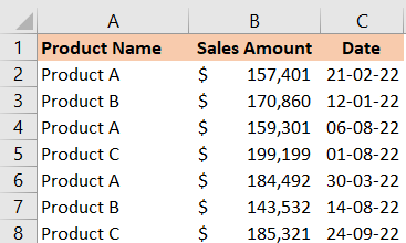
For our example, we will presume that we have a sales data table. The data will be constructed in the following way: Product Name will be in Column A, Sales Amount will be in Column B, and Date will be in Column C:
In case we want to sum all the sales of a certain product, for example, product C, we could use the SUMIF formula to achieve it. We will insert the formula in cell F2:
|
1 |
=SUMIF(A2:A8,"Product C",B2:B8) |
This formula has three parameters: range, criteria, and sum_range. Our range is A2:28, the criteria is Product C, and the sum_range will be the data in range B2:B8.
Once we insert the formula, the result will be as follows:
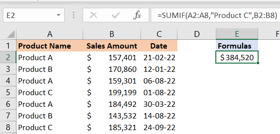
The result will be $384,520, which is the sum of cells B5 and B7, where product C is located.
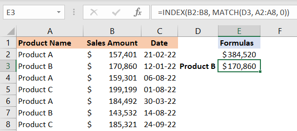
INDEX and MATCH is a more dynamic formula, but if we want to use it for similar purposes, it will not be possible, as this formula searches for the first value in our table. If we put the value Product B in cell D3, we will insert the following formula in cell E3:
|
1 |
=INDEX(B2:B8, MATCH(D3, A2:A8, 0)) |
This formula will only find the first value that is equal to Product B in our table, which will result in the number of $170,860:
SUMIF, INDEX, and MATCH Combined
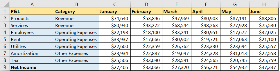
To show the full capacity of these formulas combined, we will create another table, one that will show the profit and loss for a certain company, with the revenues and expenses that will be categorized. The data will show the monthly result from every category, ranging from January to June:
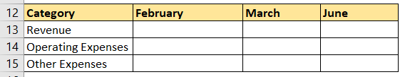
In the table below, we will extract three categories that we have: revenue, operating expenses, and other expenses, line them up in three rows, and we will use three months: February, March, and June (these will be in different columns):
We can insert only one formula to get all the results we need. The formula in cell B13, which is the result for February Revenue will be:
|
1 |
=SUMIF($B$1:$B$9,$A13,INDEX($C$1:$H$9,0,MATCH(B$12,$C$1:$H$1,0))) |
And the result will be number $147,168.
We will drag this formula in empty cells, and will get the following result:
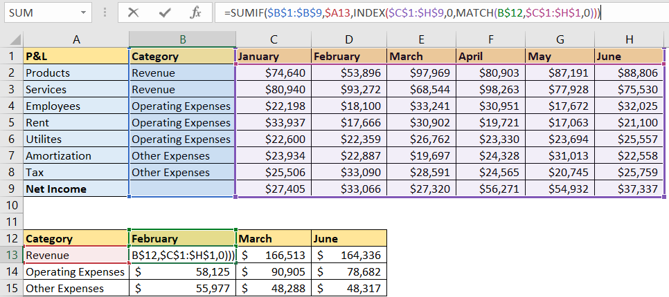
This formula is based on SUMIF. The components are:
- Range: The range will be the data in column B (B1:B9), and we will lock this table, as we will always look within these values.
- Criteria: Our search criteria will be in column A, and we will lock the column value, and change the rows as we go. This way, search criteria will vary from Revenue to Operating Expenses, and finally to Other Expenses.
- For the sum_range, we will use the data from range C1:H9, but we will do this through INDEX and MATCH, to retrieve only the values from a certain month. In the INDEX and MATCH formula, the values are:
- Range C1:H9 is used as an array;
- We put in 0 as a row number, as we already have a row value found in revenue;
- For the column number, we use the MATCH formula, for which we use the value in row 12 as a lookup_value (the row value will be locked, but the columns will change from February to March, and finally to June). Lookup_array will be range C1:H1, as we want to find the values in this range.
Combined, these formulas can give us excellent flexibility and an overview of the table, no matter how complex it is. Our example might be a little simplified, but the same formula can be applied to a larger set of data. Combined, these formulas can give us a nice flexibility and overview of the table, no matter how complex it is. Our example might be a little simplified, but the same formula can be applied to a larger set of data.