Although Excel has many built-in formulas that fall under many categories: statistical, mathematical, logical, and many more, there are some things that cannot be automatically calculated, but we have to do things manually.
Such is the case with Mood’s Median Test. This test is a non-parametric statistical test that is used to compare the medians of two or more independent samples. It is used mainly when the data that we have does not meet the assumptions of parametric tests, such as the t-test or ANOVA.
In the example below, we will show how this test can be performed in Excel.
Mood’s Median Test in Excel
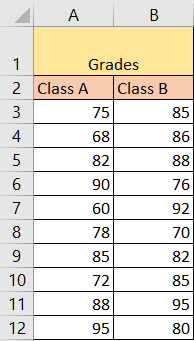
For our example, we will use two separate data sets, that will be located in columns A and B. They will show the grades of students from class A and class B:
Now we will take several steps for Mood’s Median test.
- Calculate MEDIAN
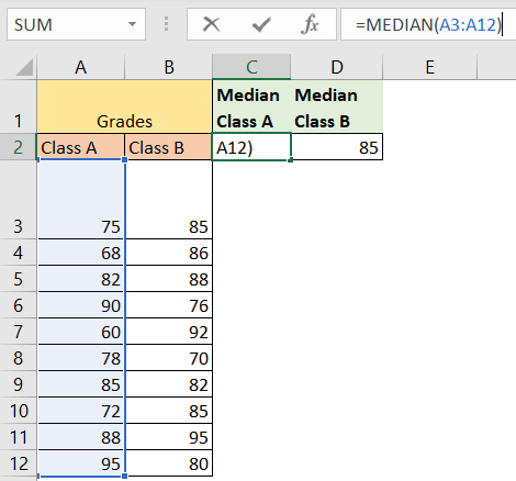
The first thing that we need to do is to calculate the medians for both classes. We will insert the data in columns C and D. In cell C2, our formula will be:
|
1 |
=MEDIAN(A3:A12) |
And we will calculate the median for column B numbers in cell D2. This is what we will end up with:
- Calculate Deviation
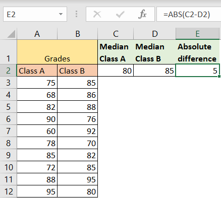
For the second step, we calculate the absolute difference between the two medians by using the following formula (located in cell E2):
|
1 |
=ABS(C2-D2) |
And will get number 5:
- Rank the data
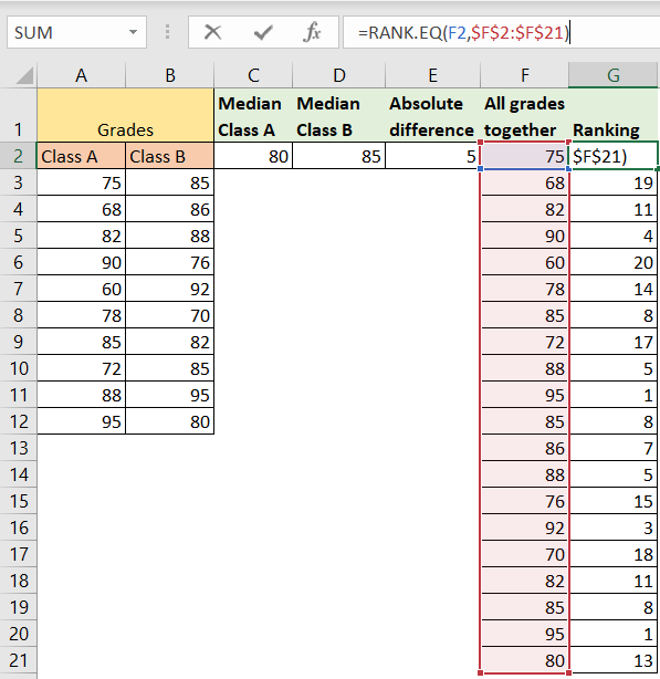
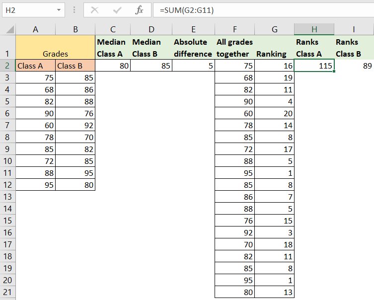
We need to rank our data, and the best way to do so is by using RANK.EQ formula. We will list all of our data in column F, and then will insert the formula:
|
1 |
=RANK.EQ(F2,$F$2:$F$21) |
In cell G2, and will drag this formula till the end of the list:
- Sum of Ranks
For the next thing, we need to sum ranks for both classes. As we are aware that the ranks for class A are located in range G2:G11, we will sum these cells and input them in cell H2. We will do the same thing for class B, and we will include the range G12:G21. The results will be 115 for class A, and 89 for class B, respectfully:
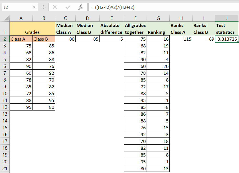
- Calculating Test Statistics
In another cell, cell J2, we will calculate the test statistic using the following formula:
|
1 |
=((H2-I2)^2)/(H2+I2) |
Which will look at the sum of ranks for class A (cell H2), and the sum of ranks for class B (cell I2). The result that we will get will be 3.31:
- Compare to Critical Value
We must look at the critical value from a Chi-Squre distribution table with 1 degree of freedom and your chosen significance level (for example, 0.05). The critical importance might be around 3.841.
- Interpretation of Results
The result obtained from the Mood’s Median Test helps us determine whether there is a statistically significant difference between the medians of the two groups. In our case, the groups are Class A and Class B, and we are comparing their student grades. Here’s what the result could indicate based on the test statistic and the critical value:
- Null Hypothesis (H0): There is no significant difference between the medians of the two groups (Class A and Class B).
- Alternative Hypothesis (H1): There is a significant difference between the medians of the two groups.
In our example, the calculated test statistic (3.31) is smaller than the critical value (3.841). What this means to us is that we do not have enough evidence to reject the null hypothesis. Therefore, the final result based on the data that we have collected, is that we cannot conclude a significant difference in medians between Class A and Class B at the chosen significance level.
The example shown here is simplified, and any real-world analysis would mean that we will probably have to reconsider assumptions, data quality, and the context in which we are working. Excel might not be the best tool for Mood’s Median Test, and some other statistical tools can probably help us more.