Using HLOOKUP in Excel to Retrieve Text Values

To retrieve text values using HLOOKUP in Excel, you must use the asterisk (*) wildcard. For example, you can use HLOOKUP with the asterisk wildcard character to retrieve the first text value in a cell range.

Note: In Excel, the asterisk (*) wildcard character stands in for any number of characters in a text string.

Explanation of HLOOKUP Function

The HLOOKUP function searches for a value in the top row of a table or range of cells and returns a corresponding value from a specified row. The “H” in HLOOKUP stands for “horizontal” because it searches horizontally across rows.

The syntax for the HLOOKUP function is as follows:

HLOOKUP(lookup_value, table_array, row_index_num, [range_lookup])

Here’s what each argument means:

• lookup_value This is the value you want to find in the top row of the table. It can be a number, text, logical value, or cell reference.
• table_array This is the range of cells that contains the data you want to search. It should include both the lookup value and the values to be returned. The table_array must have at least two rows.
• row_index_num This is the row number in the table_array from which you want to retrieve the value. The first row in the table_array is considered row number 1.
• range_lookup This is an optional argument that specifies whether you want an exact or approximate match. If set to TRUE or omitted, HLOOKUP will try to find an approximate match and return the closest value that is less than or equal to the lookup value. If set to FALSE, HLOOKUP will only find an exact match.

The following are three examples of using HLOOKUP in Excel to retrieve text values.

Example #1: Use HLOOKUP to Retrieve the FirstText Value in a Cell Range

Consider the dataset below, which displays the sales figures for different regions.

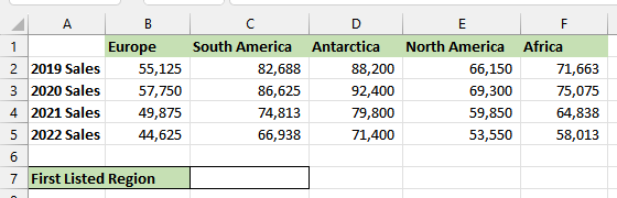
We aim to use HLOOKUP to fetch the initial region listed in row 1 and display it in cell C7.

We use the following steps:

1. Select cell C7 and type in the following formula:

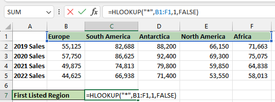
2. Press Enter.

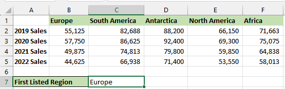
The first region listed in row 1, which is “Europe,” is shown in cell C7:

Example #2: Get The First Text Value That Starts With a Particular Letter in a Cell Range

Consider the dataset below, which presents sales figures for various regions.

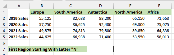
We want to use HLOOKUP to return the first text value in row 1 that starts with the letter “N” and display it in cell D7.

We use the below steps:

1. Select cell D7 and type in the below formula:

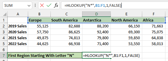
2. Press Enter.

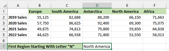
The text value in row 1 that begins with the letter “N” – North America – is shown in cell D7:

Example #2: Get The First Text Value That Ends With a Particular Phrase in a Cell Range

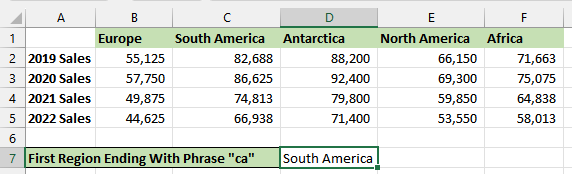
Let’s take a look at the dataset below, which displays sales data for different regions.

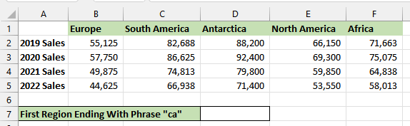
We aim to utilize HLOOKUP to retrieve the first text value in row 1 ending with the phrase “ca” and show it in cell D7.

We use the following steps:

1. Select cell D7 and type in the following formula:

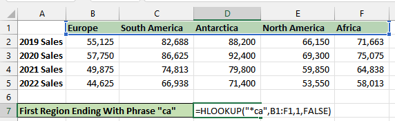
2. Press Enter.

The first text value in row 1 that ends with the phrase “ca” – South America – is shown in cell D7:

Note

Try out the XLOOKUP function, an enhanced version of HLOOKUP. Unlike HLOOKUP, XLOOKUP can be utilized in any direction, and by default, returns exact matches, making it a more user-friendly and convenient option.

Conclusion

This tutorial showed three examples of utilizing the HLOOKUP function in Excel to retrieve text values. We hope you found the tutorial helpful.