Excel offers a robust tool for filtering Pivot Tables with the VBA code. In this article, I’m going to show you different ways you can do it.
Create a Pivot table in VBA
We have the following data:
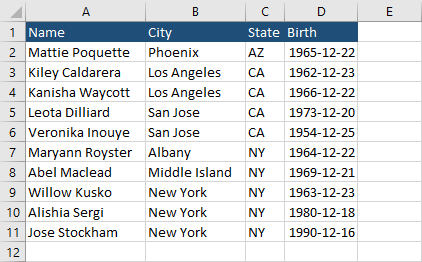
It’s a list of names with cities, states, and birth dates. I’m going to use this data to demonstrate filtering options.
Make sure that the sheet with the data is active and run this code:
|
1 2 3 4 5 6 7 8 9 10 11 12 13 14 15 16 17 |
Sub CreatePivotTable() Dim mySheet As Worksheet Dim myPivotCache As PivotCache Dim myPivotTable As PivotTable Dim myPivotTableStart As String Dim myString As String myString = ActiveSheet.Name & "!" & Range("A1:D11").Address(ReferenceStyle:=xlR1C1) Set mySheet = Sheets.Add myPivotTableStart = mySheet.Name & "!" & mySheet.Range("A1").Address(ReferenceStyle:=xlR1C1) Set myPivotCache = ActiveWorkbook.PivotCaches.Create(SourceType:=xlDatabase, SourceData:=myString) Set myPivotTable = myPivotCache.CreatePivotTable(TableDestination:=myPivotTableStart, TableName:="PivotTable1") End Sub |
In the beginning, this subprocedure gets the data range for the pivot table (A1:E11).
Next, it creates a new sheet with the default name.
The myPivotTableStart variable determines where the Pivot Table starts. In this case, it’s cell A1.
Next, we are going to create myPivotCache to hold the replica of the data source.
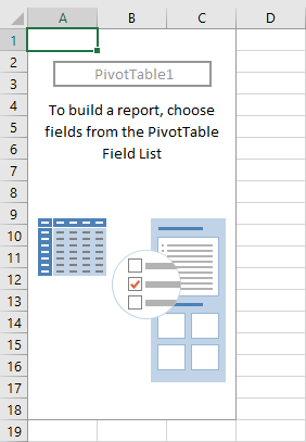
At the end of the procedure, a pivot table name “PivotTable1” will be created from this cache.
Filtering Pivot Tables
It’s time to start filtering Pivot Table data. You can assign 5 different values to a field.
| Name | Value | Field |
| xlHidden | 0 | No field |
| xRowField | 1 | Rows |
| xColumnField | 2 | Columns |
| xlPageField | 3 | Filters |
| xlDataField | 4 | Values |
The following code inserts Pivot Table elements into fields:
|
1 2 3 4 5 6 7 8 9 |
Sub AddPivotFields() Set myPivotTable = ActiveSheet.PivotTables("PivotTable1") myPivotTable.PivotFields("Name").Orientation = xlRowField myPivotTable.PivotFields("City").Orientation = xlRowField myPivotTable.PivotFields("City").Position = 1 myPivotTable.PivotFields("State").Orientation = xlPageField myPivotTable.PivotFields("Birth").Orientation = xlHiddenField End Sub |
At the beginning of the code, there is a Pivot Table assignment to the myPivotTable variable.
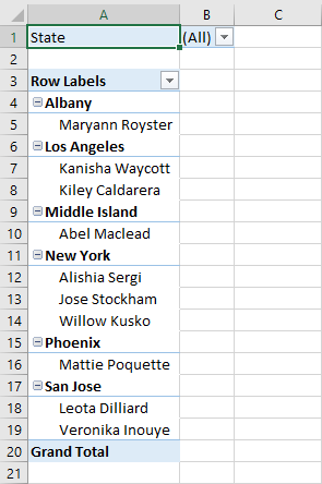
Two table headers (“Name” and “City”) are added to the Rows Field. Now, “City” is after “Name”, but it’s important to have “City” as the first position. The next line of code do just that.
The “State” field is added as a Pivot Table filter.
The last line before the end is xlHiddenField. It makes sure that the “Birth” header is not used in any field of the Pivot Table.
Clear filter
If you want to run the code multiple times, you may want to clear the Pivot Table before doing that. This code will help you with that.
Add it just after assigning a Pivot Table to a variable:
|
1 2 |
Set myPivotTable = ActiveSheet.PivotTables("PivotTable1") myPivotTable.ClearTable |
You can also create a sub procedure to do that:
|
1 2 3 |
Sub ClearPivotTable() ActiveSheet.PivotTables("PivotTable1").ClearTable End Sub |
Filter based on variable
Each person lives in a city that is located inside a state. There are codes of three states: New York, California, and Arizona. Instead of displaying all the values, display only one based on a variable:
Add Pivot Table fields again, ad run the following code.
|
1 2 3 4 5 6 7 8 9 |
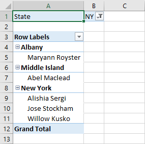
Sub FilterBasedOnVariable() Dim myPivotField As PivotField Dim filterValue As String Set myPivotField = ActiveSheet.PivotTables("PivotTable1").PivotFields("State") filterValue = "NY" myPivotField.CurrentPage = filterValue End Sub |
This code will restrict the filter to display only people and cities that are located in the state of New York.
Filter based on cell value
You can also use cell value instead of a variable. You have to add a filter value inside a cell. I added one next to the table.
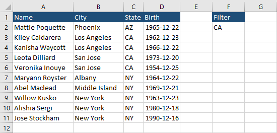
Change the filterValue variable. This is what the code looks like:
|
1 2 3 4 5 6 7 8 9 |
Sub FilterBasedOnCellValue() Dim myPivotField As PivotField Dim filterValue As String Set myPivotField = ActiveSheet.PivotTables("PivotTable1").PivotFields("State") filterValue = ActiveWorkbook.Sheets("Sheet1").Range("F2").Value myPivotField.CurrentPage = filterValue End Sub |
Now, instead of New York, we have filters or California.
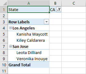
Filter on multiple items
You can also filter data using multiple values. You can use arrays or ranges.
Based on array
Code becomes more complicated when we start to deal with multiple elements. It wouldn’t be a problem if we just could set visibility to all elements to False and then add True to ones from an array. The problem is, if you try to set all visible elements to False, Excel will return an error.
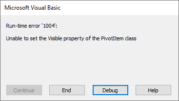
We have to do it using a different approach. First, let’s run the code.
|
1 2 3 4 5 6 7 8 9 10 11 12 13 14 15 16 17 18 19 20 21 22 23 24 25 26 27 |
Sub FilterMultipleArray() FilterArray = Array("AZ", "NY") Dim myPivotField As PivotField Set myPivotField = ActiveSheet.PivotTables("PivotTable1").PivotFields("State") myPivotField.ClearAllFilters myPivotField.EnableMultiplePageItems = TRUE numberOfElements = UBound(FilterArray) - LBound(FilterArray) + 1 If numberOfElements > 0 Then With myPivotField For i = 1 To myPivotField.PivotItems.Count j = 0 Do While j < numberOfElements If myPivotField.PivotItems(i).Name = FilterArray(j) Then myPivotField.PivotItems(myPivotField.PivotItems(i).Name).Visible = TRUE Exit Do Else myPivotField.PivotItems(myPivotField.PivotItems(i).Name).Visible = FALSE End If j = j + 1 Loop Next i End With End If End Sub |
At the beginning of the code, we have to clear all filters and enable the ability to choose multiple page items.
Now, we are using UBound and LBound functions to determine the number of elements inside the FilterArray array.
Having this number, we can use the If clause and run it only if there is at least one element inside the array (numberOfElements > 0). This assures us that there is at least one element, otherwise, it would set all values to false and therefore return an error.
Later in the code, there are two loops: For and Do While.
They are used to check each item in the filter (AZ, NY, CA) with items inside the array (AZ, NY).
If both values match, the code makes the pivot item visible and exits the loop (Exit Do) because we know that this value exists. If we didn’t exit the loop, the pivot item would be overridden by the next item in the array and the visibility would be set to False.
This is the result of the code:
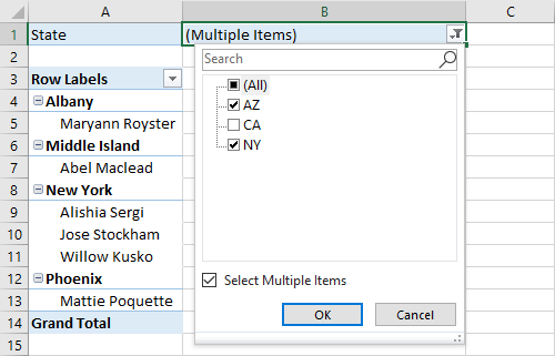
As you can see, the Select Multiple Items checkbox is selected, and both values (and only them) from the table are checked (Visible = True). Values that are not in the list are unchecked (Visible = False).
Based on the range
There is a way to use a range of cells as a source for filter items. Just be sure that these items are in one column, and that there are no empty cells anywhere.
To illustrate how it works, add one more position to the filter on “Sheet1”.

Now, you have to switch this code in “FilterMultipleArray”:
|
1 |
FilterArray = Array("AZ", "NY") |
To this one:
|
1 |
FilterArray = Application.Transpose(ActiveWorkbook.Sheets("Sheet1").Range("F2:F3").Value) |
Transposing this range converts a 2d array to a 1d array.
The rest of the code should stay the same.
