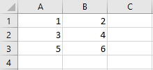
As you know, you can use the SUM function or the autosum button to sum a range inside an Excel worksheet. But you can also do it by using the VBA code.
There are a few ways you can do it. Take a look at the following examples. The sum of all cells equals 21.

Normally, you can use the following Excel function.
|
1 |
=SUM(A1:B3) |
If you want to use this range and return the value in an active cell, you have to modify the code. First, open the VBA editor by pressing Alt + F11.
Using the Excel SUM function
The easiest way to do it is to use the function we created earlier and put it into parentheses.
|
1 2 3 |
Sub SumVBA1() ActiveCell.Value = "=Sum(A1:B3)" End Sub |
If you execute this code, it will return 21.
You can also specify the row and column number.
|
1 2 3 |
Sub SumVBA2() ActiveCell.Value = "=SUM(" & Range(Cells(1, 1), Cells(3, 2)).Address(False, False) & ")" End Sub |
This time, instead of using reference, we specified a range between row 1 and column 1, and between row 3 and column 2.
Using the VBA SUM function
This time instead of using the Excel SUM function in parentheses, we will do it using the proper way, by using the VBA Sum function.
The following code is a VBA alternative of the first example.
|
1 2 3 |
Sub SumVBA3() ActiveCell.Value = WorksheetFunction.Sum(Range("A1:B3")) End Sub |
This code is the alternative to the second example, where you can specify the row and column number.
|
1 2 3 |
Sub SumVBA4() ActiveCell.Value = Application.Sum(Range(Cells(1, 1), Cells(3, 2))) End Sub |
