Once you know how to create and manipulate the data in the Excel Pivot Table, it is quite easy and self-exploratory to create various metrics and statistics from the data.
One of the things that can certainly be helpful in creating the chart from the Pivot Table.
Creating a Chart from the Pivot Table
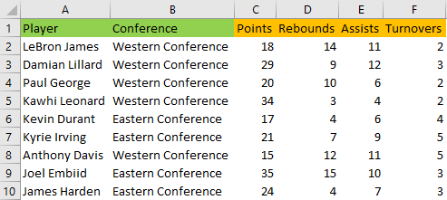
For our example, we are going to use the table with NBA players with their respecting conference and their nightly statistics for points, rebounds, assists, and turnovers.
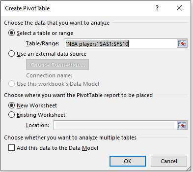
We already explained how to create a Pivot Table on various occasions. We need to select our range, go to Insert >> Tables >> Pivot Tables.
Next, we will create the Pivot Table in a new Excel sheet:
Our new sheet will be simply named “Pivot Table”.
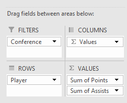
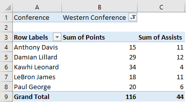
In our table, we will filter our conference to be a Western one. We will put Players in Rows fields, Sum of points, and Sum of Assists in Values fields:
Our table now looks like this:
When we click on any field in our table, PivotTable Tools will appear above the ribbon. There are two tabs in these tools: Analyze and Design.
In Analyze subtab, the PivotChart icon is located.
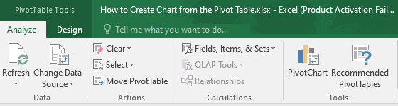
We will select our range (starting from the third row in this case) and click on the PivotChart icon. Insert Chart window will appear:
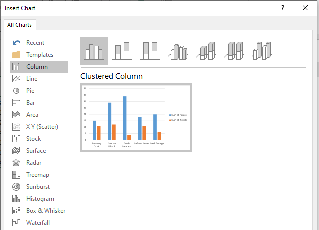
This window has numerous options for us to choose from, and they are pretty simple to use since the preview of every chart is located on the right side.
Not to complicate things too much, we will select the first one in line: Columns Chart with Clustered Column (the one in the picture above).
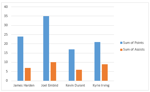
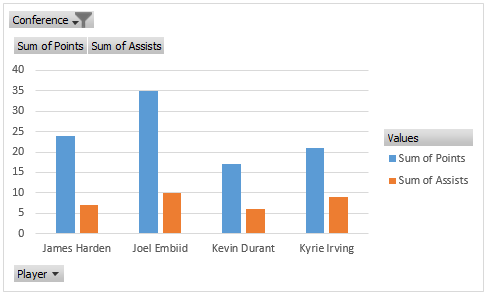
Our chart looks like this:
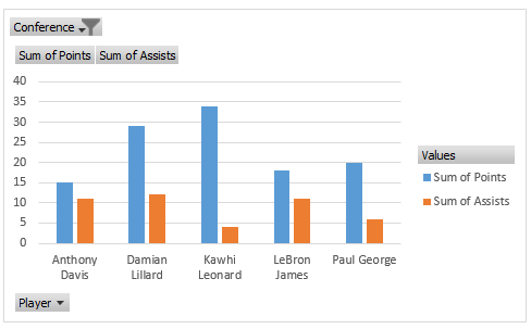
You can automatically see the difference between the regular chart and the Pivot Chart. This difference can be seen in these greyed-out fields that represent just that- Pivot Table fields.
Since the conference is our desired filter for the Pivot Table, we can easily change it in the chart. This will automatically change the data in our Pivot Table as well:
This operation functions both ways. We can either change the data in the Pivot Table or the Pivot Chart. It will not make much of the difference.
You will notice that the Player field is also greyed-out and that it has a dropdown arrow. This means we can also manipulate which player we want to include in the chart.
Although this function makes our chart interactive, some users would prefer to exclude this option, to make the chart neater.
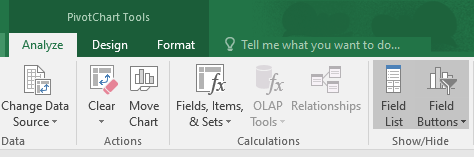
There is a solution for this as well. All you have to do is click on the chart, then go to PivotChart Tools >> Show/Hide section >> Field Buttons:
Once you click on the downward arrow, you will have a dropdown list with the following options:
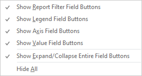
If we just click on the icon, we will hide all of our buttons, and have a clean chart: