A popular method to create a macro is to use the Macro Recorder. When you use this tool, you show Excel (by clicking on different elements in the application) the sequence of steps that it needs to perform each time you execute the macro.
Excel records every move you make, including actions such as scrolling, clicking cells, and so on. You should have your moves planned in advance when you record a macro, otherwise, you will have a lot of unwanted code.
Recording a Macro
You can record the macro in one of two ways:
- In the first method, click the button in the lower-left corner of the worksheet.

If you don’t see this icon, right-click the green area and make sure that the Macro Recording position is checked.
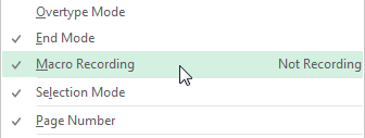
- Another method is to choose VIEW >> Macros >> Macros >> Record Macro….
When you use one of these methods, a new window will appear.
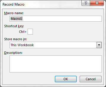
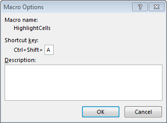
When you create a keyboard shortcut to your macro, you may want to consider using the Ctrl + Shift + letter because many keyboard shortcuts with only the Ctrl key are already taken.
TIP
Here, you can change the macro name and add a description. You can also create a shortcut key, so you will be able to execute your macro instantly.
If you choose the shortcut that is already used in Windows, it will override the default one. For example, if you use the Ctrl + N shortcut for your macro, this shortcut will only be used to execute this macro, unless you change it in VIEW >> Macros >> Macros >> View Macros >> Options ….
CAUTION
Look at the following example:
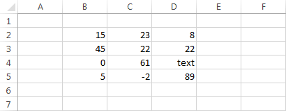
At first, it may seem that all cells, instead of D4 are numbers. But when you use the Ctrl + ` shortcut, you will notice that in fact only some of them are numbers, other are text and formulas.
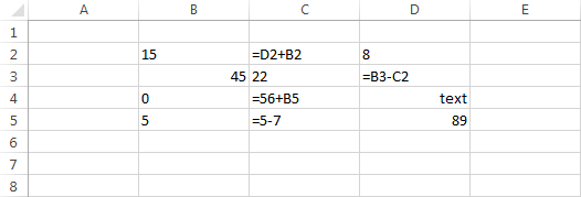
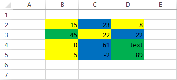
Let’s suppose that you want to create a macro that will apply to each type of data (numbers, text, and formulas) in a different color.
Because the macro recorder records your every move, you don’t want to remember moves that are not necessary. In this example we will work with the HOME tab, so make sure that you have this tab already opened.
- Click the record button, name your macro and apply a keyboard shortcut. Then choose HOME >> Editing >> Find & Select >> Go To Special and select Constants >> Numbers.
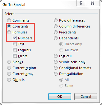
After you click the OK button all the numbers become selected.
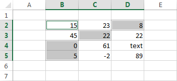
Select HOME >> Font >> Fill Color and choose the yellow color. Click outside the box to unselect cells.
- Click Go To Special and this time select Constants >> Text. Select a green color and click any cell outside the area.
- One more time choose to Go To Special, select Formulas, and check numbers. Click OK and apply the blue color.
Click the Stop icon to stop recording the macro.

If you did everything correctly, you should see the following result.
Executing the macro
Click a blank cell and select Format Painter (HOME >> Clipboard >> Format Painter). Select all highlighted cells to remove formatting and align them to the right.
Now, execute the macro using one of the three methods:
- Go to VIEW >> Macros >> Macros >> View Macros. Select the macro and click the Run button.
- Use the shortcut key (if you defined it in the Record Macro window).
- Go to DEVELOPER >> Code >> Macros.
As you can see with this macro all the highlighting can be done with just a single click.
Analyzing the Macro code
In order to preview the code generated by the macro, use the Alt + F11 keyboard shortcut.
|
1 2 3 4 5 6 7 8 9 10 11 12 13 14 15 16 17 18 19 20 21 22 23 24 25 26 27 28 29 30 31 32 33 34 |
Sub HighlightCells() ' ' HighlightCells Macro ' ' Keyboard Shortcut: Ctrl+Shift+Z ' Selection.SpecialCells(xlCellTypeConstants, 1).Select With Selection.Interior .Pattern = xlSolid .PatternColorIndex = xlAutomatic .Color = 65535 .TintAndShade = 0 .PatternTintAndShade = 0 End With Range("G8").Select Selection.SpecialCells(xlCellTypeConstants, 2).Select With Selection.Interior .Pattern = xlSolid .PatternColorIndex = xlAutomatic .Color = 5287936 .TintAndShade = 0 .PatternTintAndShade = 0 End With Range("F7").Select Selection.SpecialCells(xlCellTypeFormulas, 1).Select With Selection.Interior .Pattern = xlSolid .PatternColorIndex = xlAutomatic .Color = 12611584 .TintAndShade = 0 .PatternTintAndShade = 0 End With Range("G4").Select End Sub |
Lines 1, 34.
Opening and closing of the subroutine.
Lines 2-6.
These lines are comments. Here, by default, you can find the name and the keyboard shortcut you assigned to the macro.
You cannot change the keyboard shortcut simply by changing the text in the comments, instead, you have to go to DEVELOPER >> Code >> Macros. Select the macro and choose Options. Change the shortcut key to the new one.
CAUTION
Lines 7, 16, and 25.
This code was created when you chose HOME >> Editing Find & Select >> Go To Special … three times, selecting constants numbers, constants text, and formulas numbers.
Lines 8-14.
The With instructions will simplify your code. It allows you to refer to the object without the need for repeating the Selection.Interior part each time. If you don’t want to use the With keyword you can use the following code:
|
1 2 3 4 5 |
Selection.Interior.Pattern = xlSolid Selection.Interior.PatternColorIndex = xlAutomatic Selection.Interior.Color = 65535 Selection.Interior.TintAndShade = 0 Selection.Interior.PatternTintAndShade = 0 |
Lines 9, 18, 27.
Here, you apply the instructions saying that the cells are to be filled with a solid color.
Lines 10, 19, 28.
.PatternColorIndex = xlAutomatic means, that for the selected cells there is a specified automatic pattern to draw objects and fill cells.
Line 11.
When you chose the yellow color, Excel automatically created this line of code: .Color = 65535. That’s the index number of yellow color. You can also specify the yellow color by using: .Color = RGB(255,255,0) or .Color = vbYellow.
Lines 12, 13.
For the following properties,
|
1 2 |
.TintAndShade = 0 .PatternTintAndShade = 0 |
you can assign a number between -1 (darkest) and 1 (lightest).
We don’t want any tint and shade, so set them to 0, which is neutral.
Lines 15, 24, 33.
In VBA, you can’t select particular cells, only ranges. Range(“G8”).Select means that Excel selects range G8, which is the same as cell G8. You can choose any cell, not necessarily those selected in the code. This code is used only to deselect the cells which you selected before applying colors.
You can select only one cell, even in searched cells. Remember not to select multiple cells. If you do this, Excel will start looking only inside the selected range and not at the entire worksheet.
CAUTION
Absolute and Relative recording
By default, Excel records a macro with absolute references to cells. But sometimes you may want to create relative cell references. Please keep reading to see how these two methods differ from each other.
Absolute Macro recording
In order to record a macro in an absolute mode, follow these steps:
- Go to DEVELOPER >> Code >> Record Macro and name it „Absolute”. Click OK to start recording.
- Select cell A1 and type „Mon”.
- Select cell A2 and type „Tue”.
- Select cell A3 and type „Wed”.
- Click cell A1.
- Click Stop Recording.
Let’s take a look at the generated code:
|
1 2 3 4 5 6 7 8 9 10 11 12 |
Sub Absolute() ' ' Absolute Macro ' Range("A1").Select ActiveCell.FormulaR1C1 = "Mon" Range("A2").Select ActiveCell.FormulaR1C1 = "Tue" Range("A3").Select ActiveCell.FormulaR1C1 = "Wed" Range("A1").Select End Sub |
You can select any cell, but when you execute this macro you will always get „Mon” in cell A1, „Tue” in cell A2, and „Wed” in cell A3.
Relative Macro recording
Let’s see how the relative macro recording works.
- Activate any cell.
- Make sure that DEVELOPER >> Code >> Use Relative References is highlighted.
- Go to DEVELOPER >> Code >> Record Macro and name it „Relative”. Click OK to start recording.
- Type „Mon”.
- Select the cell below and type „Tue”.
- Select the cell below and type „Wed”.
- Click the cell where you typed „Mon”.
- Click Stop Recording.
This is the code generated by VBA:
|
1 2 3 4 5 6 7 8 9 10 11 |
Sub Relative() ' ' Relative Macro ' ActiveCell.FormulaR1C1 = "Mon" ActiveCell.Offset(1, 0).Range("A1").Select ActiveCell.FormulaR1C1 = "Tue" ActiveCell.Offset(1, 0).Range("A1").Select ActiveCell.FormulaR1C1 = "Wed" ActiveCell.Offset(-2, 0).Range("A1").Select End Sub |
Line 5.
If you execute this macro in cell C5, Excel will insert „Mon” inside the active cell (C5).
Line 6.
VBA moves the active cell one position below- to cell C6.
Lines 10.
The active cell is moved up by two cells, to cell C5.
If you didn’t start with cell A1 as a reference, it may seem strange that Excel generated such code. This is just the way that the macro recorder works.
NOTICE
Excel 365 Update
- Limited Visual Update: While the core functionality remains similar, Excel 365 offers a slightly modernized look for the Macro Recorder interface.
- Recording Still Straightforward: The process of recording macros hasn’t changed significantly. Users familiar with Excel 2016 can easily transition to recording macros in Excel 365.
- Security Enhancements: Excel 365 implements stricter security measures around macros. Macro settings might need to be adjusted to allow the running of recorded macros compared to Excel 2016.
