There are so many ways in which we can manipulate our data in Excel. One of the things that could be troublesome for you when working with a large amount of data is how to extract unique values.
There are a couple of ways to do so in Excel, and we will present them in the text below.
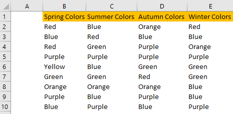
We will use a simple table of colors for our example and will create it in the sheet called Colors (a totally random name).

Extract Unique Values using Pivot Table
You may already assume that we can use an unbelievably useful Pivot Table to help us deal with this issue. But for this to work out in such a way that only the unique value is preserved, we have to do it differently than usual.
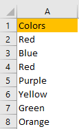
First, we have to insert a blank row in front of our data, in this case in column A. Our table looks like this:
Next, we will click on any cell in our data, then press the Alt+D combination on a keyboard, then press the P key to open the PivotTable and PivotChart Wizard.
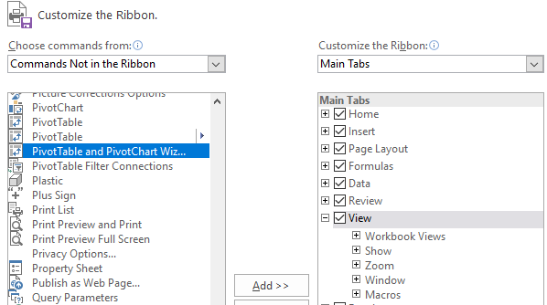
Alternatively, you can add this Wizard to your ribbon. Right-click anywhere on the ribbon and then click Customize the Ribbon.
In the Choose commands from in the dropdown list, find Commands Not in the Ribbon. From there, find the PivotTable and PivotChart Wizard and add them to your ribbon.
Once you click on this Wizard, a pop-up window with three steps will appear:
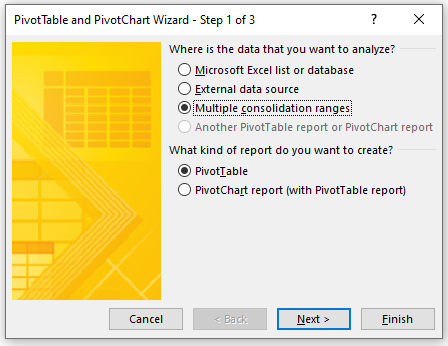
We will choose Multiple consolidation ranges and PivotTable in the first step and select Next.
In the second step, we have to click on Create a single page field for me button:
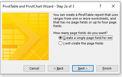
Once we click on the Next button, step 2b has to be performed. In this step, we choose the desired range.
We will select our table with data along with the new blank column that we have created (column A).
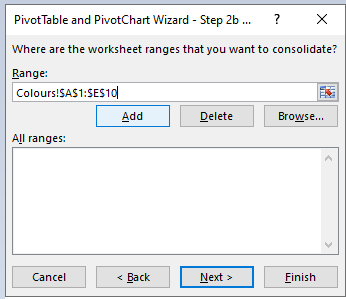
We will click on the Add button and add our range to All ranges and then click Next.
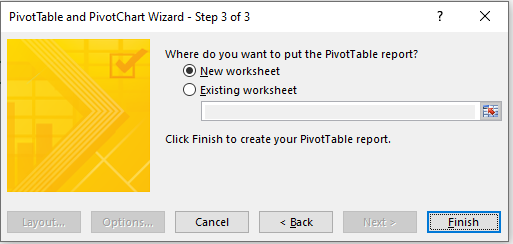
For the last step (step 3) we select where we want to place our Pivot Table. We will select New worksheet and click Finish to create a new worksheet that we will simply call “Pivot”.
We will have our Pivot Table fields automatically created.
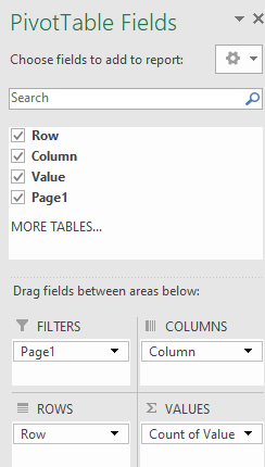
We will unselect them all to make our field list empty. Once we do that, we will drag our Value field to the Rows.
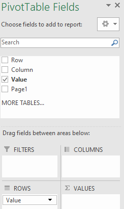
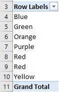
We now have our Pivot Table showing only the unique field from all of the columns:
Unique Values using Remove Duplicates
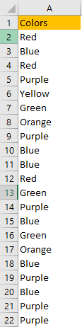
Now, there is an option that requires a little more manual work. We will take our data for this option, copy it, and then paste it onto another sheet. We will simply call our sheet „Colors 2“. Next, we are going to copy all of the data from columns B, C, and D and paste it into column A (without pasting the column names).
We will delete columns B, C, and D, and our data now looks like this:
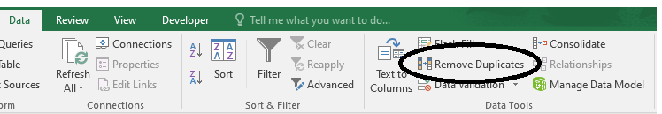
To find unique values, all we have to do is remove the duplicates. There is a great tool for this. We select column A and then go to Data >> Data Tools >> Remove Duplicates:
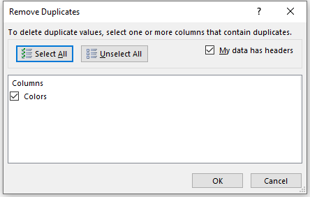
A pop-up window will appear, asking us to select the columns in which we want to find the duplicates:
We click OK and we get the following message:
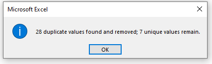
Our table now looks like this:
Extract Unique Values using the VBA code
There are also numerous ways to extract unique values from multiple columns with different VBA codes.
We will create a new Excel file- Macro enabled one, with a .xlsm extension, and copy our data in the sheet that we will also name Colors. We will create one more sheet and name it the VBA code. In this sheet, the information that we need will be extracted.
Our VBA code looks like this:
|
1 2 3 4 5 6 7 8 9 10 11 12 13 14 15 16 17 18 19 20 21 22 23 24 25 26 27 28 29 30 |
Sub unique_names() Dim data As Range Set data = ActiveSheet.UsedRange Dim column As Range, cell As Range Dim names() As Variant ReDim names(data.cells.Count) Dim i As Long i = 0 For Each column In data.Columns For Each cell In column.cells If cell.Value <> "" Then names(i) = cell.Value i = i + 1 End If Next cell Next column Dim arr As New Collection, a Set arr = unique_values(names) For i = 1 To arr.Count Worksheets("VBA").cells(i, 10) = arr(i) Next End Sub Private Function unique_values(iArr As Variant) As Collection Dim arr As New Collection, a On Error Resume Next For Each a In iArr arr.Add a, a Next Set unique_values = arr End Function |
Now, it might look like a lot, and it does take a lot of VBA knowledge to understand this code and its complexity in full. First of all, you have to be familiar with creating and adding value to your variables. Then, you have to know about For Each Next loop. Finally, you have to understand how arrays work.
We are going to step through the code to explain it in more detail:
First part:
|
1 2 3 4 5 6 |
Sub unique_names() Dim data As Range Set data = ActiveSheet.UsedRange Dim column As Range, cell As Range Dim names() As Variant ReDim names(data.cells.Count) |
In this part of the code, we are naming our code to be unique_names. Next, we are defining the variable data to represent the range and we are setting this variable to be equal to the range that we are using (UsedRange equals all of the cells that are filled in a worksheet).
Furthermore, we are declaring two more variables: column and cell (they are also range objects) and we are declaring an array called names to be the type of Variant (this type is used for all variables that we did not explicitly declare).
We then resize our array (names) by the ReDim statement. Since this array was formally declared, we are now changing it to correspond to all of the cells from our data variable (i.e. all the cells that are filled in a worksheet).
|
1 2 3 4 5 6 7 8 9 10 |
Dim i As Long i = 0 For Each column In data.Columns For Each cell In column.cells If cell.Value <> "" Then names(i) = cell.Value i = i + 1 End If Next cell Next column |
In this part, we are defining the new variable (i) which is defined as a number (Long is used to storing very long numbers, from -2,147,483,648 to 2,147,483,648).
We first hardcode this variable to be equal to 0.
Our goal is to populate our names array. We create two nested For Each loop. The first one looks into each cell in our columns, checks if the value is different than empty then populates our names array (first cell in the array, then all the others) with that is equal to the cell value. This is done only if the condition about the cell not being empty is met.
The second For Each loop is the one on top. After the first one is executed (checks all the cells in the first column) this one starts and moves to a different column. When it goes to a different column, the first loop is started again.
This is repeated until our array called names is populated with all the cells that are in our active sheet (sheet Colors).
|
1 2 3 |
Dim arr As New Collection, a Set arr = unique_values(names) |
For the next part, we have to extract all the unique values from our array. For this, we have to declare a new collection. Collections are an excellent way of storing a group of items together. In Excel, a good representative of the collection is workbooks or worksheets.
We then set this collection to be equal to unique_values (names, in our case).
Since unique_values does not exist, we created a new function that can be called, as follows:
|
1 2 3 4 5 6 7 8 |
Private Function unique_values(iArr As Variant) As Collection Dim arr As New Collection, a On Error Resume Next For Each a In iArr arr.Add a, a Next Set unique_values = arr End Function |
This function creates unique_values as a collection, with the iArr parameter as a Variant. Then it creates another collection that is called arr.
It then searches for a parameter “a” in collection unique_values and adds that value to our arr collection.
“a” basically represents a variable that will get all of the values from our worksheet.
Then it sets unique_values to correspond to arr collection. This way, it only finds those values that are equal in both collections, and it finds them only once.
|
1 2 3 4 |
For i = 1 To arr.Count Worksheets("VBA").cells(i, 10) = arr(i) Next |
For the last part, the code is to copy the values from arr collection into our sheet called VBA. These values will be in column J.
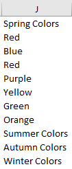
Notice that even the name of the columns is transferred, as these are unique values as well.
Keep in mind that this code is pretty hard to understand, and to do so, you have to have a very good knowledge of arrays and collections, in the first place. We will discuss those in different examples.